
This is the first part of the Portfolio Optimization with Python series. The intend is to make a deep dive into the field and study some real-world applications with Python. Throughout the series, I’ll be using MOSEK library for solving the optimization problems and Backtrader for backtesting the portfolio management strategies.
This time, I’ll make a brief introduction to the Markowitz Portfolio Optimization framework so you start to familiarize with the relevant concepts. At the end, I’ll show you a simple function building the Markowitz Mean-Variance portfolio using MOSEK and finding the optimal weights and efficient frontier.
Markowitz Portfolio Optimization
Let’s consider an investor who wishes to allocate capital among \(N\) securities at time \(t=0\) and hold them over a single period of time \(t=h\). Moreover, assume that the investor is risk-averse, that is, he/she is looking to maximize the return of the investment while trying to keep the investment risk on an acceptable level. We can think of the risk as the uncertainty of the future portfolio returns.
The investment risk can be decomposed into two components: the specific risk and the systematic risk. We can’t do much with the systematic risk part: the only way of reducing it is by decreasing the expected return of the portfolio. On the other hand, the specific risk, or the risk associated with each of the securities in the portfolio, can be reduced through diversification for a fixed expected return. Markowitz Theory (also known as Modern Portfolio Theory) formalizes this process by using the variance as a measure of portfolio risk, and constructing an optimization problem whose solution are the optimal portfolio weights for the given inputs and constraints (more on this later).
Before I go any further, let me define some important quantities:
- \(p_{0,i}\): the known price of a security \(i\) at the beginning of the investment period.
- \(P_{h,i}\): the random price of the security \(i\) at the end of the investment period \(h\).
- The rate of return of the security \(i\) over the investment period \(h\), modeled by the random variable
\[R_{i}=\dfrac{P_{h,i}}{p_{0,i}}-1\]
- The expected value of the rate of return of the security \(i\)
\[ \mu_{i} = \mathbb{E}(R_{i}) \]
- The portfolio vector \(\mathbf{x}\in\mathbb{R}^{N}\), where \(N\) is the number of symbols and \(x_{i}\) is the proportion of funds invested into security \(i\).
- The random portfolio return
\[R_{\mathbf{x}}=\sum_{i}^{N}x_{i}R_{i}=\mathbf{x}^{T}R,\]
where \(\mathbf{R}=[R_{1}, \dots, R_{i}, \dots, R_{N}]^{T}\) is the vector of asset’s returns.
- The expected portfolio return
\[\mu_{\mathbf{x}}=\mathbb{E}(R_{\mathbf{x}})=\mathbf{x}^{T}\mathbb{E}(R)=\mathbf{x}^{T}\mathbf{\mu},\]
where \(\mathbf{\mu}\) is the vector of expected returns.
- The portfolio variance
\[\sigma_{\mathbf{x}}^{2} = \text{Var}(R_{\mathbf{x}}) = \sum_{i}^{N}\text{Cov}(R_{i}, R_{j})x_{i}x_{j}=\mathbf{x}^{T}\mathbf{\Sigma}\mathbf{x},\]
where \(\mathbf{\Sigma}\) is the covariance matrix of returns.
Based on these quantities, we can state the portfolio optimization problem defined above as
\[\begin{array}{lr}\text{minimize} & \mathbf{x}^{T}\mathbf{\Sigma}\mathbf{x}\\ \text{subject to} & \mathbf{\mu}^{T}\mathbf{x} \geq r_{min} \\ & \mathbf{1}^{T}\mathbf{x} = 1\end{array}\]
That is, minimize the variance of the portfolio given a minimum required portfolio return \(r_{min}\) and the budget constraint \(\mathbf{1}^{T}\mathbf{x} = \sum_{i}^{N} x_{i} = 1\), which means that the portfolio is fully invested. Given this, the optimization problem is also referred as Mean-Variance Optimization (MVO).
Using the input parameters \(\mathbf{\mu}\) and \(\mathbf{\Sigma}\), MVO seeks to find a portfolio of assets \(\mathbf{x}\) in such a way that it seeks the optimal trade-off between expected portfolio return and portfolio risk. There are two alternative formulations to the problem statement given above:
- Maximize expected return for a risk level
\[ \begin{array}{lr} \text{maximize} & \mathbf{\mu}^{T}\mathbf{x} \\ \text{subject to} & \mathbf{x}^{T}\mathbf{\Sigma x}\leq \gamma^{2} \\ & \mathbf{1}^{T}\mathbf{x} = 1,\end{array} \]
where \(\gamma^{2}\) is an upper bound on the portfolio risk.
- Maximize the utility function of the investor
\[ \begin{array}{lr} \text{maximize} & \mathbf{\mu}^{T}\mathbf{x} - \dfrac{\delta}{2}\mathbf{x}^{T}\mathbf{\Sigma x} \\ \text{subject to} & \mathbf{1}^{T}\mathbf{x} = 1,\end{array} \]
where \(\delta\) is the risk-aversion coefficient. The problem with this formulation is that the risk coefficient does not have an intuitive investment meaning for the investor. However, if we reformulate the problem using the standard deviation
\[ \begin{array}{lr} \text{maximize} & \mathbf{\mu}^{T}\mathbf{x} - \tilde{\delta}\sqrt{\mathbf{x}^{T}\mathbf{\Sigma x}} \\ \text{subject to} & \mathbf{1}^{T}\mathbf{x} = 1,\end{array} \label{9} \]
and assume that the portfolio return is normally distributed, then \(\tilde{\delta}\) is the z-score of portfolio return, that is, the distance from the mean measured in units of standard deviation. We can see that for \(\tilde{\delta}=0\), we maximize expected portfolio return. Then, by increasing \(\tilde{\delta}\), we put more and more weight on tail risk, i.e., we maximize a lower and lower quantile of portfolio return.
All the formulations above will result in the same set of optimal solutions. The optimal portfolio \(\mathbf{x}\) is said to be efficient in the sense that there is no other portfolio giving a strictly higher return for the same amount of risk (variance). The collection of such points (portfolios) is known as the efficient frontier in the mean return-variance space.
We can use the method of Lagrangian multipliers to obtain a closed-form solution for the optimization problem above. However, in the investment practice it is common to include additional constraints in the form of linear and convex equalities or inequalities. Examples of constraints are diversification constraints, leverage constraints, turnover constraints, among others. Furthermore, extra objective function terms can be included for representing restrictions on the optimal weights. In these more realistic use cases, it is compulsory to use numerical optimization algorithms for finding the optimal solution.
Diversification constraints
We will focus our attention on diversification constraints, which help to limit portfolio risk by restricting the exposure to individual positions or sectors.
For a single position \(i\), we have
\[ l_{i} \leq x_{i} \leq u_{i}, \]
where \(l_{i}\) is the lower bound and \(u_{i}\) the upper one.
On the other hand, for a sector or group of assets \(\mathbb{I}\), we have
\[ l_{i} \leq \sum_{i\in\mathbb{I}}x_{i}\leq u_{i} \]
Note that the constraints of the type greater than (similar for constraints of the type less than) that apply to all the assets can be expressed in matrix form as
\[ \mathbb{I}^{N\times N} \mathbf{x} \leq \mathbf{1}_{N} u \]
where \(\mathbb{I}^{N\times N}\) is the identity matrix with \(N\) columns and rows, \(\mathbf{1}_{N}\) is an \(N\)-dimensional vector of ones and \(u\) is the upper bound.
Additionally, greater than constraints (similar for less than constraints) for assets in a specific sector can be expressed as
\[ \mathbf{1}_{i\in\mathbb{I}}^{T}\mathbf{x} \leq u \]
where \(\mathbf{1}_{i\in\mathbb{I}}^{T}\) is an \(N\)-dimensional vector whose values are \(1\) if the asset \(i\) belongs to the sector \(\mathbb{I}\) or \(0\) if not.
Finally, greater than (or similarly less than) constraints for a specific asset can be expressed as
\[\mathbf{1}_{i=j}^{T}\mathbf{x} \leq u \]
where \(\mathbf{1}_{i=j}^{T}\mathbf{x}\) is an \(N\)-dimensional vector whose values are \(1\) only for the asset \(j\) of interest
Conic formulation
The portfolio optimization problems stated above are quadratic optimization (QO) problems. Solving QO in their original form is popular and considered easy. However, more recent results showed that conic optimization models can improve QO models both in the theoretical and in the practical sense.
Conic (quadratic) optimization, also known as second-order cone optimization, is a straightforward generalization of linear optimization, meaning that we optimize a linear function under linear (in)equalities with some variables belonging to one or more quadratic cones.
An \(n\)-dimensional quadratic cone is defined as
\[ \mathcal{Q}^{n} = \left\{ x \in \mathbb{R}^{n} | x_{1} \geq \sqrt{x_{2}^{2} + x_{3}^{2} + \cdots + x_{n}^{2}} \right\} \]
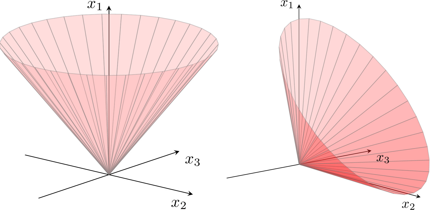
Example of the geometric interpretation of a quadratic cone and a rotated quadratic cone (not discussed here) with three variables. source
Having this in mind and assuming that the covariance matrix \( \mathbf{\Sigma} \) is positive definite such that
\[ \mathbf{\Sigma} = \mathbf{G}\mathbf{G}^{T}, \ \ \ \mathbf{G}\in\mathbb{R}^{N\times k}\]
we can write the portfolio variance as
\[ \mathbf{x}^{T}\mathbf{\Sigma x} = \mathbf{x}^{T}\mathbf{G}\mathbf{G}^{T}x = ||\mathbf{G}^{T}\mathbf{x}||_{2}^{2}. \]
We can find the conic equivalent of the problem in Eq. \( (\ref{9})\) by introducing a variable \(s\) to represent the upper bound of the portfolio standard deviation, and model the constraint \( ||\mathbf{G}^{T}\mathbf{x}||_{2}\leq s \) using the quadratic cone as
\[ \begin{array}{lr} \text{maximize} & \mathbf{\mu}^{T}\mathbf{x} - \tilde{\delta}s \\ \text{subject to} & \left(s, \mathbf{G}^{T}\mathbf{x}\right) \in \mathcal{Q}^{k+1} \\ & \mathbf{1}^{T}\mathbf{x} = 1 \label{15} \end{array} \]
Solving the problem in this format will result in a more robust, faster and reliable solution process.
Python implementation
Enough theory for now, let’s code! We’ll be using MOSEK’s Fusion API for solving the optimization problem. MOSEK is an interior-point optimizer for linear, quadratic and conic optimization problems that is employed by several technological, financial and educational institutions. Fusion is an object-oriented API designed for building conic optimization models in a simple and expressive manner.
In the Fusion API, the user’s interface to the optimization problem is the Model object. The Model class is used for
- formulating the problem by defining
Variables,Parameters, constraints and the objective functions, - solving the problem and retrieving the solution status and solutions,
- interacting with the solver.
Let’s define a function for building a Fusion Model that represents the problem from Eq. \( (\ref{15})\). The function will receive the following inputs:
n_assets: number of assets in the investment universe.asset_sectors: pandasDataFramecontaining a column with the assets names ("Asset") and another with their corresponding sector ("Sector").constraints: List of constraints. The constraints will be dictionaries containing the following keys:"Type": type of constraint. It can be"All Assets"(the constraint applies to all the assets),"Sectors"(the constraint applies only to assets from a particular sector) or"Assets"(the constraint applies to a particular asset)."Weight": limit value for the assets’ weights."Sign": domain of the constraint. It can be">="(greater than) or"<="(less than)."Position": indicates to which positions the constraint applies. It can be the name of a sector, the name of an asset or an empty string ("") if the constraint type is"All Assets".
You’ll find examples of asset_sectors and constraints below.
| |
Let me walk you through the code above:
- Line 15 instantiate the
Modelobject. - Lines 18 and 21 create the optimization variables
x(portfolio weights) ands(upper bound of the portfolio variance). For creating a variable, we first need to pass the variable’s name, then the dimension (1for scalars) and lastly, the domain. The domain can beunboundedif there is no restriction; orgreaterThanorlessThanif there are lower and upper bounds. - Lines 24 and 27 create the parameters for the covariance matrix decomposition
Gand the expected returns vectormu. We will later set the values of these parameters using real data. Defining bothGandmuas parameters is very handy because we can compare different estimation methods without the need of re-building the model. As you can see, parameters are created in a similar way than variables, passing first the name and then the dimension. - Line 30 defines the
deltaparameter for the objective function. We will later try different values for it. Note thatdeltais a scalar, so we don’t need to pass the dimension in this case. - Line 33 set the budget constraint. A constraint is set by passing the name, the mathematical expression and the domain (equality or inequality). Note that the Fusion API has several expressions for performing summation, simple and matrix multiplication, dot product, etc. You can see a complete list in Section 6.3 of MOSEK’s documentation.
- Lines 36 through 83 set the constraints by asset/s and sector/s.
- Lines 86 through 93 set the conic constraint for the portfolio variance. Note that
Gis not transpose here, so we will need to take care of this when setting its value. - Lines 96 through 103 define the objective function of the problem.
Now, let’s define the investment universe and grab some historical data from Yahoo Finance for estimating the covariance matrix and the vector of expected returns. We will use the yfinance package for downloading the data.
| |
For now, we will use the sample estimates for the covariance matrix and expected returns vector. We will see in later posts how we can improve the estimation of these input parameters, which is an important topic because the optimization is highly sensible to them. The covariance matrix decomposition will be computed using the Cholesky’s decomposition.
| |
We’ll impose the following constraints:
- No asset will take more than \(20\%\) of the portfolio.
- We want to invest at least \(30\%\) and no more than \(40\%\) of our wealth in the Electronic Technology sector.
- We don’t want META to take more than \(5\%\) of the portfolio.
- We want to invest no more than \(10\%\) in Crypto.
The python version of this constraints is as follows:
| |
We are now ready to build the model, set the values of the required parameters and solve the optimization problem. We’ll set delta=0.1. For the sake of comparison, we will also solve the unconstrained problem (only considering no short-selling).
| |
In the figure below, we can see that the constrained version selected a greater amount of assets and assigned lower weights to them, which helps to improve portfolio diversification.
Additionally, we can easily check that all the constraints are met.
Finally, we can compute the efficient frontier by solving the problem for different values of delta.
| |
Hover your mouse over the plot and zoom-in to see the weights of each portfolio in the frontier.
Conclusion
In this post we went through the fundamental concepts of Markowitz Portfolio Optimization and solved the constrained mean-variance optimization problem with the help of MOSEK’s Fusion API. By using real market data, we confirmed that including weight constraints helps to improve portfolio diversification (and thus lowering specific risk). In the next posts, we will solve a different problem: maximize portfolio’s risk-adjusted return measured by the Sharpe Ratio. Additionally, we will perform a backtesting to analyze strategy’s performance. You can find the full code here in the markowitz_mv.ipynb notebook. Stay tuned for more!